Inverse Schelling

In 1974, economist Thomas Schelling proposed an agent-based simulation as a model of how segregation inadvertently arises in communities. Suppose one places two kinds of tokens on the squares of a chess board. Let a token’s “neighbors” be the spaces up, down, left, right, and diagonally adjacent. A token, or “agent,” is satisfied in Schelling’s model if at least a given percentage of its neighbors are of the same type as itself (the same color token, for instance). If it is unsatisfied, it must be moved somewhere else on the board. Schelling’s discovery was that even with a seemingly low threshold such as 30%, colors begin to clump together almost immediately, with surprisingly little intermixing. This is often taken as an analogy for segregation in housing markets, with “agents” as homeowners, and with the startling implication that even if we are satisfied to be in the minority, we may still unwittingly segregate ourselves. The simulation at left runs a version of Schelling's original model. The simulation can be reset to a random distribution by clicking on the frame and pressing "r." I implemented Schelling’s Model to test it for myself, and by tweaking a few important parts of his algorithm I found an equally interesting inverse phenomenon. Suppose an agent is satisfied only if at least some percent of its neighbors are unlike itself. Under this condition, instead of clumps, a pattern of stratified lines quickly emerges. This pattern can be seen as a way of mixing two equal populations so that they come into maximum contact. For comparison, in this sense it outperforms even the seemingly well-mixed checkerboard pattern. Below, the first example is Schelling's original model, while the second is the model inverted.

A traditional Schelling simulation after several rounds, showing signs of stabilization

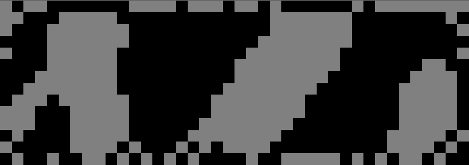
A mostly stabilized inverted model showing striated patterns

Inverted model showing striated patterns

Inverted model showing striated patterns

More recently I have been interested in the fact that the inverse model appears to reach an ordered state more quickly than the traditional model. In an effort to quantify this, I set the grid to 100x100, and plotted the satisfaction rate--the percentage of grid cells satisfied at a given timestep--for 100 or 10000 timesteps. The apparent distinction between the two models is visually confirmed by these plots. Moreover, we note that (A) the rate of convergence is higher in the inverse model, as demonstrated by the greater slope of its curve in the log-log plot (B) while both models fluctuate more as time goes on, the inverse model is stabler, exhibiting smaller fluctuations So a population of agents all seeking local heterogeneity will be more satisfied, more quickly, than one made up of agents all seeking local homogeneity.

100 steps; linear scale

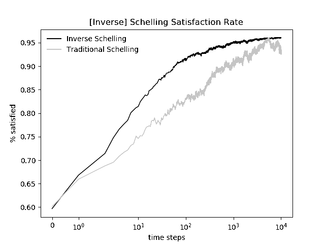
10000 steps; log-log scale